Why the Excel Vlookup Function is “So Last Year, Darling” – Part 2

In my last blog, I showed you how easy it was to use Power Pivot to produce a Pivot table that pulled in data across two tables, Drinks and Categories (without using a Vlookup). Well, we’re going to carry on ditching the Vlookup by looking at Power Pivot’s equivalent function, called “Related”
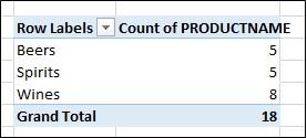
Remember in our fictitious wine bar (in down town Billingshurst) we were able to find out that we stock most drinks that are from the “Wines” category;-
But let’s face it, what we really want to know is what our sales are and where we can make the most profit selling our drinks.
Let’s bring some customers into the Billingshurst Bar scenario. Here they are:-
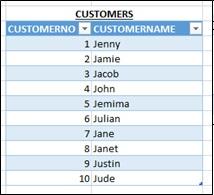
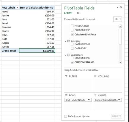
We want to find out how much each Customer has spent at our Bar.
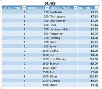
And just to remind you, these are the drinks we’re selling.
Both these tables have been imported into Power Pivot by firstly formatting the data as a Table and then using the “Add to Data Model” icon on the Power Pivot tab.
In my last blog, I showed you how in the Power Pivot window you could link two tables together by using a column that was common to both (i.e. CategoryNo in the Categories table to CategoryNo in the Drinks table). But notice in our two tables, Customers and Drinks, there is no common column (try saying that when you’ve drunk too much Chardonnay!)
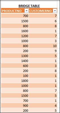
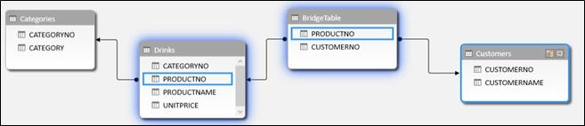
Because there are no columns in common across our tables, we can’t link our customers together with their drinks so we need another table to record each drink that our customers have bought. We’ll call this table “BridgeTable” (because we’re bridging customers to their drinks). The BridgeTable only needs two columns; ProductNo and CustomerNo and looks like this. (I’ve just shown you a few rows of data so you get the idea):-
Notice we use ProductNo and CustomerNo in our BridgeTable, not the names of things (only because we’re not very good at spelling – is that “Lagar” I see in the Drinks table?)
In the Diagram View in the Power Pivot window, we now join Customers to the BridgeTable and Drinks to the BridgeTable because we now have columns common to both tables.
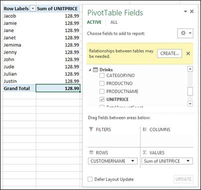
We want to know how much each customer has spent. Now this is where it’s all likely to go pear shaped. If we bring UnitPrice down from the Drinks table and put it in the Values area of the Pivot Table, it doesn’t work (unless they’ve all spent £128.99 which would be extremely unlikely):-
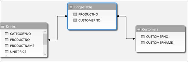
The problem is that where you have tables related together in one-to-many relationships (in Diagram View, the arrow points towards the “one” side of the relationship), you can only place fields from the “many” side into the Values area of the Pivot Table and the UnitPrice fields comes from the Drinks table which is on the one side:-
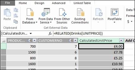
The solution is quite simple. I’m sure you’re thinking that if you were using Excel, you would use a Vlookup to pull the UnitPrice into the BridgeTable using the ProductNo field as the Lookup Value. We can do a similar thing in Power Pivot but it is MUCH simpler than a Vlookup. Just open up the Power Pivot window and in the BridgeTable add a new column by double clicking where it says “Add Column”. Give your column a name (e.g. CalculatedUnitPrice) and enter this formula:-
=RELATED(DRINKS[UNITPRICE])
Now all you need to do is bring this column into the values are of the Pivot Table.
Now, I’ve been around for a long time, I’ve got a lot of miles on the clock you might say. I’ve used Vlookup, Hlookup and just Lookup. I’ve used CountIf, Countifs, Sumif and Sumifs. I’ve use Match and Index and more Excel functions than I care to remember. But they’re all now just…..well…..so LAST YEAR DARLING.
Add new comment