Blog

The following is an extract from Alison's book 'Up and Running with DAX for Power BI'. 

For many DAX users, getting to grips with the concept of table expansion is the final piece in the jigsaw of understanding how DAX works. The reason for this is that good data modelling practice results in filters only propagating from the one side of a relationship to the many.  When this happens, most people assume that relationships between tables use “primary” and “foreign” keys to perform “lookups” from dimension tables to the fact table to enable filtering.  This is probably how you think filter propagation works.  It’s not that this theory is wrong, it’s just that it’s not complete. 

What is Table Expansion?

When a measure is evaluated, many-to-one relationships allow table expansion to take place. Table expansion results in the creation of virtual tables by the DAX engine that include the columns of the base table but also then expand into all the columns from related tables on the one side of the relationship.  The DAX engine then uses the expanded table to group by values in the expanded table’s columns and apply filters accordingly.   Therefore, every table has a matching expanded version of itself that is generated in memory that contains all its own columns plus any columns from tables that are related to it, that are on the one side of the relationship either directly or indirectly.  Relationships only exist to generate expanded tables.

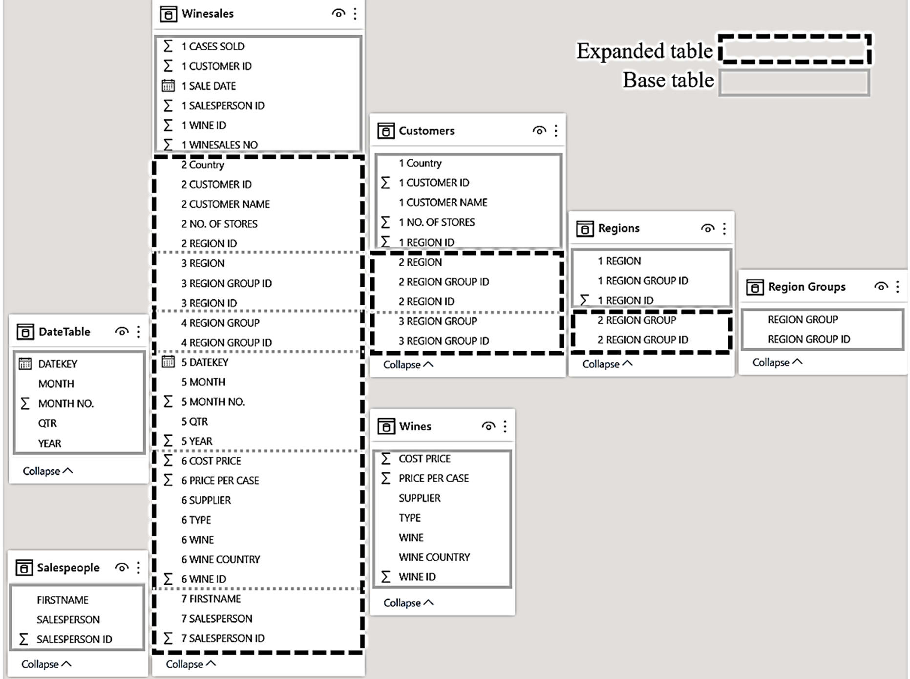
Therefore, we can now talk about both base tables and expanded tables in a data model.  Base tables are just that, the tables.  Expanded tables are the base tables that also contain all the columns from tables that are related to them.  Let’s take the data model shown below as an example.  You can see that it comprises the following:-

1. A “Winesales” fact table.
2. "Wines", “Salespeople”, “Customers” and “DateTable” dimensions.
3. The “Regions” and “Region Groups” tables that snowflake from the Customers table.

Image

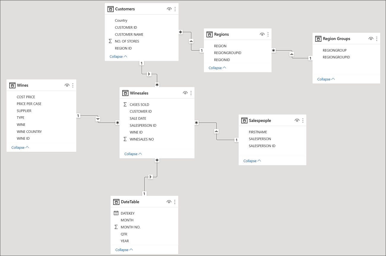
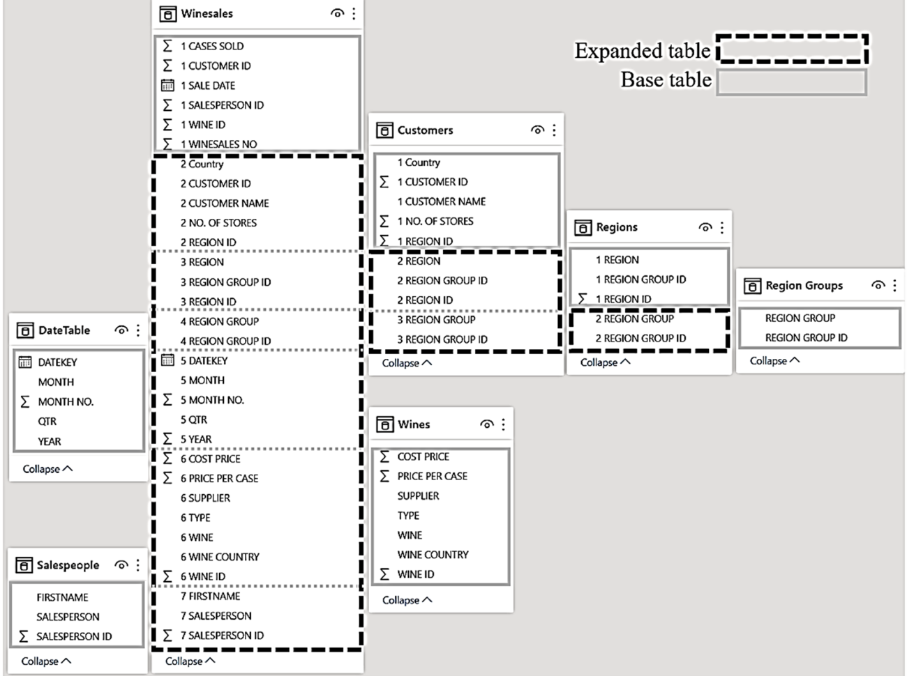
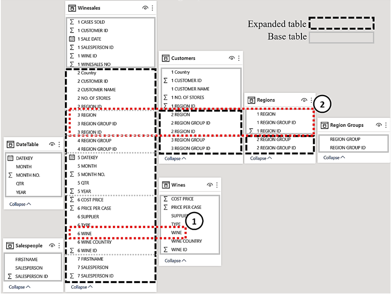
In this model we have three tables that will expand; Winesales, Customers and Regions.  The Winesales expanded table will contain all the columns from all the tables in the model.  The Customers expanded table will include all the columns from the Regions dimension and the Region Group dimension.  The Regions expanded table will include all the columns from the Region Group dimension. We could therefore redesign our data model to show what it might look like in memory on the evaluation of a measure. Notice there are no relationships between the tables because relationships only exist to generate expanded tables:-

Image

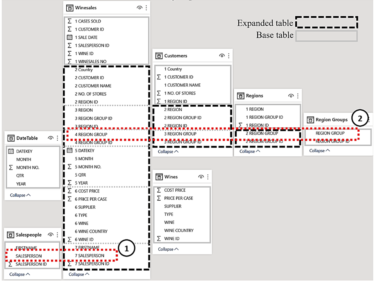
Once a filter is applied to a column, all the expanded tables containing that column are also filtered.  For example, we can see below that filtering the SALESPERSON column from the Salespeople base table filters the Winesales expanded table ( 1 ) and filtering REGION GROUP column from the Region Groups base table filters the Regions expanded table, the Customers expanded table and the Winesales expanded table ( 2 ).

Image

Relationships exist only to expand tables; they are not used to filter them.  Any reference to a table in a DAX expression is always a reference to the expanded table, where applicable.

Another important aspect of table expansion is that when we use ALL inside CALCULATE to remove filters from a table, it removes filters from the expanded table, if applicable.  This includes any columns from dimensions related to the expanded table and therefore includes columns where the filter was originally generated.  So, the expression “ALL (  Winesales )” will remove any filters from any of the base tables related to Winesales, which includes the entire data model.

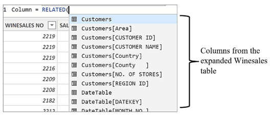
Understanding table expansion means we can clarify certain behaviours in DAX. For example, we can describe accurately how the RELATED function works.  RELATED doesn’t “lookup” values in related tables but instead allows you to find columns that already exist in the expanded table.  When you use RELATED on the fact table for instance, you are shown all the columns from the expanded fact table in the IntelliSense list:-

Image

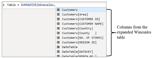
Like RELATED, the ALLEXCEPT and SUMMARIZE functions also allow you to use the columns in expanded tables.  When constructing an expression using these functions, if you reference a fact table or a snowflake dimension, you are again presented with all the columns from the expanded table in the IntelliSense list:-

Image

You may be thinking that knowledge of table expansion is purely theoretical. It explains certain behaviours regarding filter propagation but doesn’t lead you forward in constructing more complex DAX expressions. For the most part, the reason you will use table expansion in your expressions is to “reach” dimensions to perform aggregations on the filtered data within them.  Without referencing an expanded table, there are two strategies you can use if this is your goal.  You can use the CROSSFILTER function to reverse the direction of filter propagation or you might use the RELATED function to pull values from dimensions into the fact table  However, neither of these approaches is best practice.  You should be using table expansion.

“Reaching” Dimensions

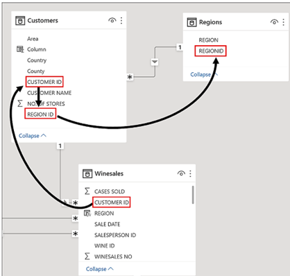
Let’s see how table expansion can allow you to break free from the limitations imposed on you by star and snowflake schemas. For example, we have been asked to calculate in how many different regions we’ve sold each wine.  The Regions table is a snowflake dimension. It is related to the Customers table that’s in turn related to the Winesales fact table. Currently, the only way we can deduce in which region a sales transaction was made is through the Customers table:-

Image

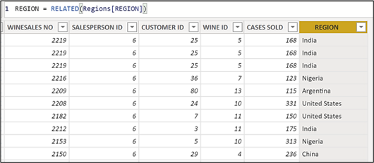
We now know however, that all the columns in the Regions table are also in the expanded Winesales table. Therefore, one approach would be to create a calculated column in the Winesales base table using RELATED to reference the REGION column from the expanded Winesales table:-

Image

You could then write the “Distinct Regions” measure using DISTINCTCOUNT on this calculated column:-

Distinct Regions =
DISTINCTCOUNT ( Winesales[REGION] )

We can see the evaluation of this measure in a Table visual that includes the WINE column from the Wines dimension:-

Image

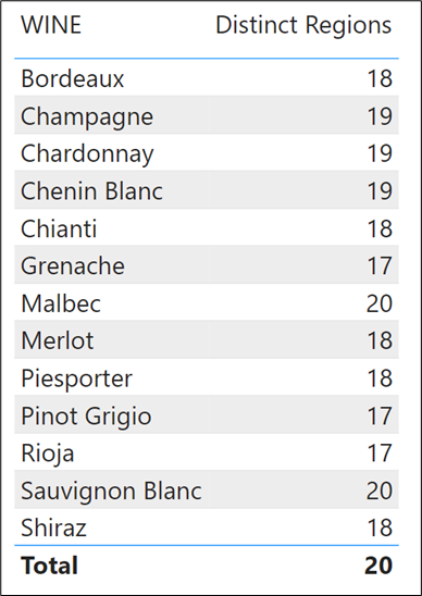
However, all that’s happening here is that you are accessing the REGION column in the expanded Winesales table and besides which, calculated columns should be avoided if possible.  There is a better way to calculate the distinct number of regions in which we’ve sold each wine and that is to use CALCULATE with a table filter that will filter the regions table to contain only those regions in which we’ve sold each wine.

When you reference a table in the filter argument of CALCULATE (explicitly or using a table expression), this will always be the expanded table, where applicable. Therefore, we can use the expanded Winesales table (that contains the REGION column) as the filter argument for CALCULATE.  This will filter the Regions table according to the rows in the Winesales expanded table that have been filtered for each wine.   This would be the measure:

Distinct Regions =
CALCULATE ( COUNTROWS ( Regions ), Winesales )

Please note the simplicity of this expression but the complexity of the concept that lies behind it; with DAX the devil is always in the detail.  Looking at the data model below, we can see that the WINE column in the Wines table filters the WINE column in the expanded Winesales table ( 1 ). The expanded Winesales table contains all the columns in the Regions table.  The filter in the expanded Winesales fact table is used to filter the Regions table whose rows are then counted ( 2 ):-

Image

The takeaway from these examples is that using an expanded table in the filter argument of CALCULATE enables you to pass filters into dimension and snowflake tables, in effect reversing the direction of filter propagation.  This is because the expanded table contains the columns from these dimensions that can then be grouped and filtered.  However, a question that must now be answered is; what is the difference between using expanded tables and using CROSSFILTER?  Isn’t the result of using these different methods the same?  For instance, we can author this expression using an expanded table:-

Distinct Regions =
CALCULATE ( COUNTROWS ( Regions ), Winesales )

Or we can author this measure using CROSSFILTER that we might assume would return the same result:-

Distinct Regions #2 =
CALCULATE(COUNTROWS(Regions),
    CROSSFILTER(Winesales[CUSTOMER ID],
       Customers[CUSTOMER ID],both),
    CROSSFILTER(Customers[REGION ID],
       Regions[REGION ID],both)   )

Both these measures will “reach” the Regions table.  Clearly, the second measure is a great deal clumsier than the first, but is there a difference in the evaluation?  The answer is, yes there is, and we will now explain why.

Table Expansion vs. CROSSFILTER

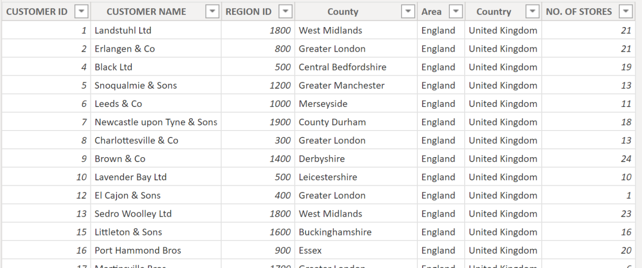
To explore this, let’s look more closely at the Customers dimension.  We can see that we have recorded the NO. OF STORES each customer owns in which we sell our wines. 

Image

We want to find out the total number of stores in which we have sold each wine.  This measure…

Total No. of Stores =
SUM ( Customers[NO. OF STORES] )

… won’t work:-

Image

The problem is that filters don’t flow from the Wines dimension through to the Customers dimension, so here we could use the CROSSFILTER function to programmatically change the direction of the filter propagation to a bi-directional filter:

Total Stores =
CALCULATE
    SUM ( Customers[NO. OF STORES] ),
    CROSSFILTER ( Winesales[CUSTOMER ID],
    Customers[CUSTOMER ID], BOTH )  )

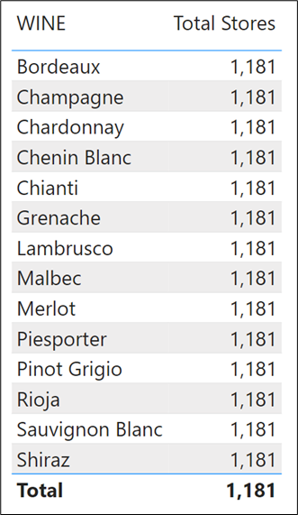
However, this measure returns an incorrect value on the Total row:-

Image

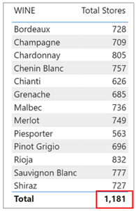
Many of the same customers will have bought each wine, so we know that the total of 1,181 will not be the sum of the values above.  However, you might think this value looks about right and so believe it.  The value in the Total row should be the total number of stores in which we’ve sold all our wines.  This value is not correct because in the Customers table we have five customers to whom we’ve sold no wines.  If we “show items with no data” in a Table visual where we calculate the “Total Sales” measure, we can see who they are:-

Image

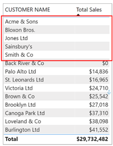
There are five customers to whom we’ve sold no wines. The value of 1,181 shown in the Total row includes the stores for these customers. We can see these values in the Customers table in the NO. OF STORES column:-

Image

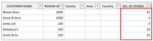
We haven’t sold any wine to these customers so clearly their stores shouldn’t be included in the Total number of stores in which we’ve sold our wines.  Our total is out by 69. 

What’s happening here is that the “Total Stores” measure uses a bi-directional filter.  When it arrives at the evaluation of the Total row, the filters are removed from the WINE column of the Wines dimension, and therefore, there is no filter to propagate to the Customers dimension.  With no filters propagated, it sums all the values in the NO. OF STORES column.   In other words, bi-directional filters are only active if filters are active. 

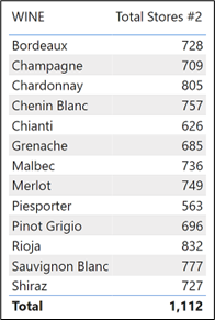
So, how do you calculate the correct value of 1,112 in the Total row? 

What you must do here is use the expanded Winesales fact table as the filter for the Customers table.  This is because, unlike bi-directional filtering, filters from expanded tables are always active.  When the Total row is evaluated, the expanded Winesales fact table contains only those Customers who have bought wines and so this will filter the Customers dimension accordingly.

This is the measure that will give you the correct total:-

Total Stores #2 =
CALCULATE (
    SUM ( Customers[NO. OF STORES] ),
    Winesales  )

The total row now shows 1,112

Image

When working with DAX, not only must you have to have an eye for detail and a suspicious mind, but you must also understand table expansion.