Context Transition: Where the Row Context Becomes a Filter Context

“Nothing in life that’s worth anything is easy.” Barack Obama.

And we could also say that nothing in DAX that’s worth anything is easy! Certainly the concept of context transition is one of the more challenging concepts to get to grips with in DAX. It can’t be explained in a few short paragraphs so I apologise in advance for this rather long blog but please stick with it and read on because once you understand this concept, a whole range of tricky calculations become possible. In fact, most DAX expressions you meet will probably be using context transition and indeed, there will come a time when most DAX expressions you write will use it.

The starting point in understanding context transition is understanding the difference between the two evaluations contexts used by DAX expressions; row context and filter context, so let’s now look at both of these in turn.

Row Context

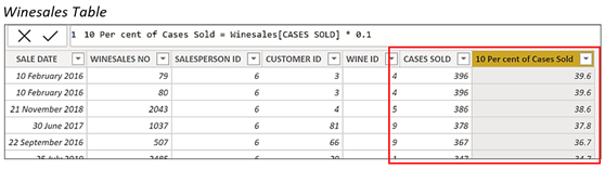
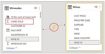
When using row context, a DAX expression iterates over every row in a table. The values used in the expression are the values sitting in the current row, which may be different for every row e.g. For example, this calculated column in the “Winesales” table…

10 Per cent of Cases Sold = Winesales[CASES SOLD] * 0.1

…will iterate over all the rows in the table, usually finding a different value for CASES SOLD on each row and multiplying it by 0.1 as shown below:-

So we know that calculated columns are evaluated in the row context. But measures will
also use the row context if they iterate a table.
So for example this measure…

Total Sales =
SUMX ( Winesales,
Winesales[CASES SOLD] * RELATED ( Wines[PRICE PER CASE] )
)

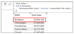
.. when put into this table visual is evaluated as follows:-

Firstly it uses the filter context to filter “Bordeaux” wine in the first instance (shown in red above).
Then the SUMX function iterates the Winesales table and using the row context, multiplies the CASES SOLD value sitting in each row by the PRICE PER CASE value from the Wines table (the Wines table is related to the Winesales table in a one-to-many relationship so we can use the RELATED function here).
Lastly SUMX sums the result of all these row-level calculations, for example for “Bordeaux” wine.

So what we can say so far is that any DAX expression that iterates over a table, whether in a calculated column or inside a measure, uses the row context.

Filter Context

All DAX measures are evaluated in a filter context. The filter context is normally generated from whatever is happening in the Power BI report when the measure is evaluated i.e. the structure of the visual, any slicers affecting the visual and any filters in the filters pane.

Note: If you’re a bit hazy on how filter context works, please read my blog that provides a comprehensive explanation: DAX “Filter Context” Explained | Power BI | Burningsuit

But there is another way a filter context can be generated and that’s what we’re going to explore now.

Where a Row Context becomes a Filter Context

There is a specific situation where a DAX expression will turn the row context into a filter context. This is what we know as “context transition”. To understand what this specific situation is exactly, let’s consider these five DAX expressions, two calculated columns and three measures (you don’t need to know at this point what the expressions do):-

These are the calculated columns:-

Column 1 = CALCULATE ( SUM ( Winesales[CASES SOLD ) )

Column 2 = [Total Cases]

These are the measures:-

Measure 1 = AVERAGEX ( Wines, [Total Cases])

Measure 2 = AVERAGEX ( Wines, CALCULATE ( SUM ( Winesales[CASES SOLD ) )

Measure 3 = CALCULATE ( [No of Sales], FILTER (Winesales, [Total Cases] > 350)

Question; what is common to all these expressions? The answer is as follows:-

Firstly, they all use the CALCULATE function. But surely Column 2 and Measure 1 don’t? At this point, there’s something more we need to say about measures. All measures implicitly invoke CALCULATE even if they don’t use the function explicitly. Therefore, Column 2 and Measure 1, which both reference the measure “Total Cases”, are both calling CALCULATE implicitly. The other expressions are using CALCULATE explicitly.

Secondly, they all iterate tables creating a row context. Columns 1 and 2 are calculated columns and all calculated columns iterate tables. We know that the functions AVERAGEX and FILTER are both iterators so Measures 1, 2 and 3 all iterate tables too, creating a row context. Measures 1 and 2 iterate the Wines table and Measure 3 iterates the Winesales table.

Thirdly, they all invoke context transition where the row context generated by either the calculated column or in the measure is turned into a filter context.

So the specific situation we alluded to above is this; context transition is invoked whenever we use CALCULATE either explicitly or implicitly AND the expression (either in a column or in a measure) iterates a table.

Okay, so this is when context transition happens, but what exactly is “context transition”? To answer this question, let’s first take this expression as a calculated column:-

Total Cases Column = SUM ( Winesales[CASES SOLD] )

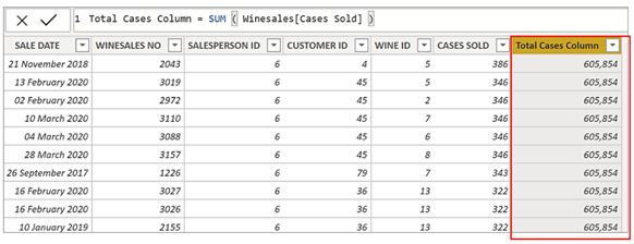
You can see that for every row it returns the same value which is the grand total of CASES SOLD. As a calculated column, it’s iterating the table using the row context and so there’s no filter present. Aggregate functions such as SUM, by definition, require that the rows to be aggregated must first be filtered. Because there is no filter on the table, this expression can only use the values from the entire table and so sums all the values for CASES SOLD.

Remember we said that context transition happens when there’s an iteration and we use CALCULATE. So let’s now take our first look at context transition in action in a calculated column by editing our expression and wrapping CALCULATE around it:-

Total Cases Column =
CALCULATE (
SUM ( Winesales[CASES SOLD] )
)

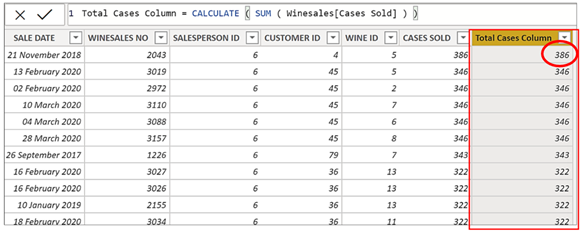
We can see that this expression returns the CASES SOLD value of each row.

What has happened here is that like all calculated columns, the expression generates an iteration over the table. But we’re also using CALCULATE and by doing so, the expression ignores the row context and replaces it with a filter context. But what is the filter? Notice that in this CALCULATE expression there are no filter arguments, so what is the filter being used by CALCULATE? The answer is rather a strange one; it’s each value in each of the columns sitting in the current row. For example, in the first row of the table where the calculation returns 386 (circled), the filter is this:-

SALE DATE = 21 November 2018
WINESALES NO = 2043
SALESPERSON ID = 6

CUSTOMER ID = 4
WINE ID = 5
CASES SOLD = 386

This is why were you to have a complete duplicate of the first row in the above example, you would see 772 (386 x 2) in “Total Cases Column” because the duplicate rows would be grouped before CASES SOLD was summed. However, each of our rows is unique so each filter generated by the context transition returns one row, that is the current row.

So our calculated column iterates the Winesales table and because of CALCULATE context transition occurs, so every single row becomes filtered out in its own right. Therefore the CASES SOLD summed are the cases sold sitting in each row. This is an example of using CALCULATE in a calculated column where we have a row context and so context transition is invoked.

However, context transition is also invoked whenever you use a measure within a row context, for example, if you put a measure into a calculated column. This is because all measures use CALCULATE implicitly and so context transition will occur. Let’s take this measure:-

Total Cases = SUM ( Winesales[CASES SOLD] )

And let’s edit our calculated column to do the same calculation but this time expressed as this measure (coloured yellow):-

Total Cases Column = [Total Cases]

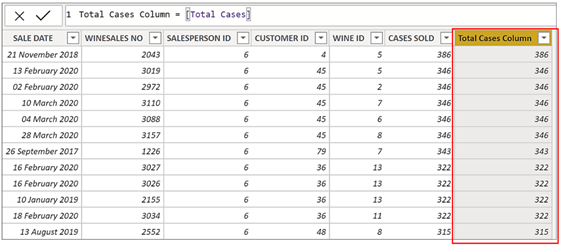
You can see the result is the same as when we used CALCULATE explicitly.

At this stage, I bet you’re thinking, why would I want to create a calculated column that returns the same value as the value sitting in the row? Also, our Winesales table, being the fact table could potentially contain millions of rows so any context transition occurring in a calculated column would be very slow. In short, what is the use of context transition?

To answer this question, let’s see how context transition works when used in dimension tables, rather than in the fact table. You can see below that the Wines dimension is related to the Winesales fact table in a many-to-one relationship:-

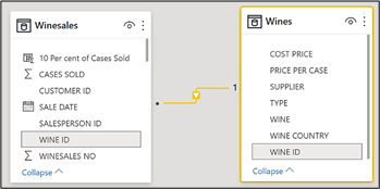
So let’s now repeat the same expressions we’ve used in a calculated column but this time in the Wines dimension rather than the fact table.

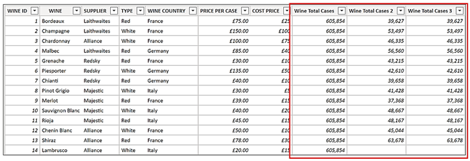
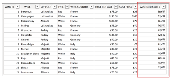
Here are the calculated columns we’ve now created in the Wines dimension:-

Wine Total Cases = SUM ( Winesales[CASES SOLD] )

Wine Total Cases 2 =
CALCULATE (
SUM ( Winesales[CASES SOLD] )
)

Wine Total Cases 3 = [Total Cases]

You can see these calculated columns in Data View in the Wines dimension shown below:-

Let’s look more closely at the evaluation of each of these calculated columns. First up is this one:-

Wine Total Cases = SUM ( Winesales[CASES SOLD] )

This calculated column uses an expression, not a measure, and it’s not using CALCULATE either implicitly or explicitly. The expression uses the SUM function that requires a filter context. In the absence of any filter it sums the CASES SOLD values in all the rows of the Winesales table giving us the grand total of CASES SOLD.

Next, let’s look at this calculated column:-

Wine Total Cases 2 =
CALCULATE (
SUM ( Winesales[CASES SOLD] )
)

The second of our calculated columns is using CALCULATE that turns the row context invoked by the calculated column into a filter context. At this point, we need to remind ourselves that the filter context always propagates through the entire Data Model. The filter context coming through from context transition behaves no differently from a filter context coming through from a visual or a slicer on the report canvas. When our expression evaluates the first row of the Wines dimension it turns the entire row into a filter that filters “Bordeaux” wine. We could imagine that in-memory, our wines dimension looks like this:-

Note: Because we can’t “see” these in-memory filters, I’ve coloured the in-memory filtered Wines table yellow to distinguish it from what you see in Data View.

What’s happening has the same effect on the table as if we had filtered “Bordeaux” in a slicer or any other means by which we could filter “Bordeaux” in a report. We know that because the Wines dimension is related to Winesales fact table in a many-to-one relationship, this filter generated by context transition, is propagated onward to the Winesales fact table.

So our Winesales fact table is now cross filtered for “Bordeaux” wines and the CASES SOLD (shown in red above) are summed for “Bordeaux” wine.

So a calculated column that uses CALCULATE where context transition is invoked behaves just like a measure in a visual on the report canvas.

Lastly, we have this calculated column:-

Wine Total Cases 3 = [Total Cases]

Looking at the third of our calculated columns, here we’re using a measure that defines the same expression as in “Total Cases 2” remembering that all measures implicitly invoke CALCULATE . “Total Cases 2” and “Total Cases 3” are the same expressions. Whenever you see a measure, even if it doesn’t use CALCULATE, you should always imagine that it’s wrapped inside CALCULATE.

How Context Transition Can Return “Surprising Results”

We’ve been using calculated columns to see context transition in action. However, we don’t need to “see” context transition to understand that it happens and besides which, you’re probably not going to be creating these types of calculated columns in reality.

Mostly context transition happens behind the scenes, in memory, when we construct iterating measures that reference another measure in the iteration (because all measures implicitly call CALCULATE). Typically it’s when we use measures inside the “X” aggregate functions like AVERAGEX or MAXX or we use measures inside the FILTER function. Because we can’t “see” context transition happening, being oblivious of its existence means we’ll struggle to understand how DAX works. Marco Russo and Alberto Ferrari in their “Definitive Guide to DAX” explain it like this:-

“Being ignorant of certain behaviors can ensure surprising results. Nevertheless, once you master the behavior, you start leveraging it as you see fit. The only difference between a strange behavior and a useful feature – at least in DAX – is your level of knowledge.”

Marco and Alberto talk about “strange behaviours” and “surprising results”. The only reason these behaviours would seem strange or surprising is that we don’t understand the behaviour of context transition; the fact that inside measures there’s a world of difference between iterations referencing measures and iterations referencing expressions. To illustrate this we’re going to look at some expressions where getting it right i.e. do you use a measure or do you use an expression, is key. In these examples, we’re going to see how DAX expressions can return “surprising results” unless of course, you understand the behaviour of context transition.

Calculating a Value Greater than an Average

In the first example, we must reference an expression in our measure to get the correct calculation, nesting the measure (that defines the same expression) won’t do.

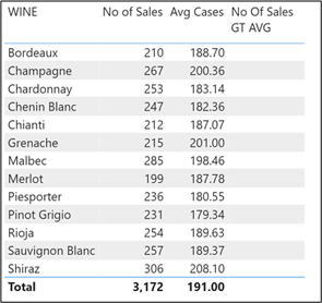
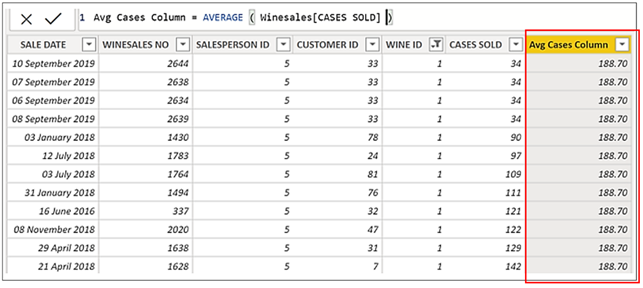
Let’s pretend that we want to calculate the number of sales for each wine where the CASES SOLD is greater than the average CASES SOLD for that wine. For example, the average cases sold for Bordeaux is 188.70 and we want to calculate how many sales of Bordeaux have CASES SOLD greater than this value (this is purely an intellectual exercise and not a particularly realistic calculation).

First, we’ve created these two measures:-

Avg Cases = AVERAGE ( Winesales[CASES SOLD] )

No of Sales = COUNTROWS ( Winesales )

Now to calculate the number of sales where CASES SOLD is greater than the average cases, we’ve created this measure:-

No Of Sales GT AVG =
VAR MyTable =
FILTER ( Winesales, Winesales[CASES SOLD] > [Avg Cases] )
RETURN
CALCULATE ( [No Of Sales], MyTable )

Note how we use the measure called “Avg Cases” (highlighted in yellow) inside the FILTER function. Also notice that In this measure, we use the FILTER function to iterate the Winesales table. We’ve placed all three of these measures in the table visual below. You can see that the “No Of Sales GT AVG ” returns nothing, a surprising result, I think you’ll agree.

Let’s look more closely at what’s happening here. This measure uses the FILTER function that iterates the Winesales table to filter out rows where CASES SOLD is greater than the value calculated by the “Avg Cases” measure. What is the value calculated by the “Avg Cases” measure? If we put this measure into the Winesales table as a calculated column, we can “see” what the FILTER function is testing the CASES SOLD against:-

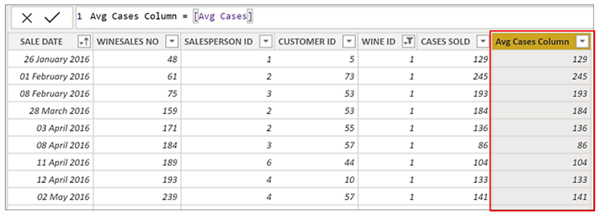
Note: Remember that the Winesales table will be cross filtered for “Bordeaux” wine in the first evaluation because of the filter context.

Because “Avg Cases” is a measure, it invokes context transition, creating a filter on each row of the Winesales table in memory. Because each row is unique, it calculates the average of the CASES SOLD only for the current row which is the same as the CASES SOLD value. Therefore the “Avg Cases” measure is never greater than CASES SOLD. You could test this out by changing “>” to “>=” where instead of blanks being returned, you would get the same values as “No of Sales”.

Let’s now replace the measure with the expression that calculates the average, and we’ll get the correct result:-

No Of Sales GT AVG =
VAR MyTable =
FILTER ( Winesales, Winesales[CASES SOLD] > AVERAGE ( Winesales[CASES SOLD] ) )
RETURN
CALCULATE ( [No Of Sales], MyTable )
)

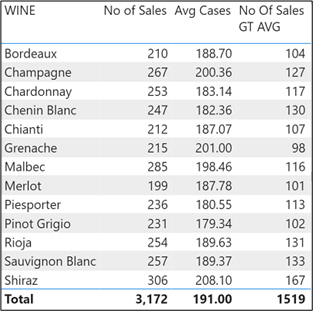
So again, to see what’s happening, if we put this expression into a calculated column shown below (rigged slightly to show what’s happening in memory for “Bordeaux” wine), we can “see” what it returns. It’s the average of all the cases sold in the Winesales table in the current filter context e.g. the average cases sold for “Bordeaux” which is 188.70. So in the first calculation for “Bordeaux”, there are 104 sales that have cases sold greater than 188.70.

Leveraging Context Transition: Finding the Maximum and Average of Totals

The real power of context transition comes when you use it to calculate averages, maximums and minimums of totals as opposed to row-level values. This is where the importance of having clearly defined dimension tables comes to the fore because to do this type of calculation, we need to use context transition on dimension tables.

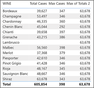
For example, take these two simple measures:-

Total Cases = SUM ( Winesales[CASES SOLD] )

Max Cases = MAX ( Winesales[CASES SOLD] )

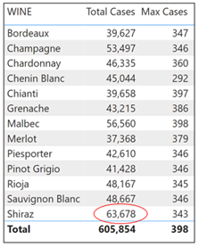
The “Max Cases” measure tells us the maximum number of cases in any single transaction in the Winesales table for each wine. For example, for “Bordeaux”, the maximum cases in any single transaction is 347 cases. However, we want to calculate the maximum of the “Total Cases” measure, i.e. 63,678 for Shiraz (circled in red).

To do this we need to use context transition.

We know that context transition is invoked in a measure that is iterated over a table. We looked earlier at creating a calculated column in the Wines dimension that used a measure to invoke context transition and so found the total cases sold for each wine:-

Wine Total Cases 3 = [Total Cases]

Rather than putting this measure into a calculated column to invoke the context transition, we could put this measure into another measure that iterates the Wines dimension to do the same. If we do this, context transition will happen in memory and we can find the maximum of these values. Let’s look at this measure:-

Max of Totals = MAXX ( Wines, [Total Cases] )

Note: In these examples, we’re using MAXX because it’s easier for you to see the calculations being done. We could equally substitute AVERAGEX or MINX to find the average or minimum of the totals.

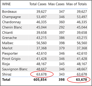
The MAXX function iterates the Wines dimension in memory to calculate the “Total Cases” measure for every row in the dimension, just like the calculated column above. It then finds the maximum of these values. But why does the “Max of Totals” measure return the same result as the Total Cases measure except in the Total Row? Let’s now answer this question.

In the first evaluation, “Bordeaux” is in the current filter context so there’s only one value for Total Cases i.e. the Total Cases value for “Bordeaux”. The maximum of only one value is that value and that’s why we see the same value for “Total Cases” and for “Max of Totals”. It’s not until the measure reaches the evaluation for the Total row, where there is no filter on the Wines dimension, that it can then find the maximum of all the wines, which is 63,678 for “Shiraz” (circled in red).

This is why, if we want to calculate the maximum of the totals for all the wines (for example to compare the maximum against the other totals), we need to remove the filter from the Wines dimension by using ALL or ALLSELECTED as in this example:

Max of Totals 2 =
MAXX (
ALL ( Wines ) , [Total Cases] )

Of course, you now get the same value against every wine! What good is that? Well, normally the context transition calculation is performed in memory to find a value that can be used by the expression. We don’t need to see the values context transition returns. So for instance, we could filter the wine that held the maximum cases sold:-

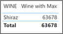
Wine with Max =
VAR MyMax =
MAXX ( ALL ( Wines ), [Total Cases] )
RETURN
CALCULATE ( [Total Cases], FILTER ( Wines, [Total Cases] = MyMax ) )

And now we can show the wine with the maximum in a visual:-

Yes, I know you could simply use a TopN visual filter to do this job. The reason we’ve used the MAXX function here is to make it easier for you to see the values being calculated by the context transition. Let’s use AVERAGEX instead to find the average of the totals, which is a better example:-

Average of Totals =
AVERAGEX ( ALL ( Wines ), [Total Cases] )

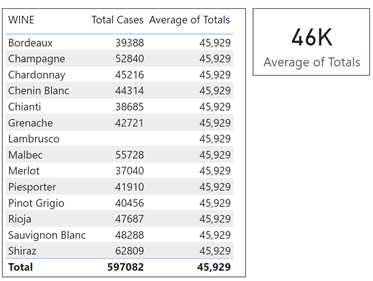
And now I can put the Average of Totals into a Card Visual and use it to show the sales performance of my wines. Any wines with a Total Cases value that is greater than this average are performing well. This is probably much more insightful than simply the average across all transactions.

We’re only scratching the surface of what can be done using context transition. You’ll find your own reasons to use it and hopefully you will no longer find the behaviour of context transition in any way “strange” or “surprising” and that’s because you now understand it.

Happy DAXing!

Blog